Introduction
- PCR (Principal Component Regression)
- PCA followed by mulitple linear regression (onto the principal component)
- Can resolve complex mixtures of neurochemicals and analyze features such as concentration or phasic and tonic fluctuations
- Deep Learning (CNN in this paper)
- Good at discovering intricate structure in high-dimensional data, mixed data and data with many similarities.
- In the case of single analyte, PCR and Deep Learning showed similar performance, but in the case of mixtures, Deep Learning showed better performance
Result and Discussion
- The regression result showed that the estimation accuracy of the four neurotransmitters using deep learning was more accurate by reducing RMSE 5-20% than using PCR for mixture data
- Estimate 300nM concentration
| |
DA |
EP |
NE |
5-HT |
| PCR |
4.28 |
1.57 |
10.97 |
2.45 |
| DL |
7.37 |
5.67 |
4.18 |
3.3 |
| |
DA |
EP |
NE |
5-HT |
| PCR |
4.61 ± 1.03 |
4.6 ± 1.1 |
6.83 ± 2.6 |
3.18 ± 0.55 |
| DL |
3.77 ± 0.41 |
3.69 ± 0.84 |
2.49 ± 0.42 |
2.67 ± 0.56 |
| |
DA + EP |
DA + NE |
DA + 5-HT |
EP + NE |
EP + 5-HT |
NE + 5-HT |
| PCR |
17.75 ± 2.86 |
20.22 ± 3.7 |
15.84 ± 1.96 |
14.24 ± 2.16 |
13.47 ± 2.38 |
19.49 ± 4.79 |
| DL |
10.17 ± 1.2 |
12.29 ± 1.71 |
11.95 ± 1.42 |
7.97 ± 1.31 |
7.73 ± 1.15 |
11.98 ± 1 |
- DL is more suited to the analysis of mixtures of neurochemicals
- DA, EP, NE and 5-HT shows the linear relation with concentration and the oxidation current at the peak potential
Limitation
- It would be necessary to improve the method related to signal reconstruction in consideration of calculating the reliability of in vivo experiments for both acute and chronic recordings
Materials and Method
In Vitro Experiments for the Deep Learning Model Validation
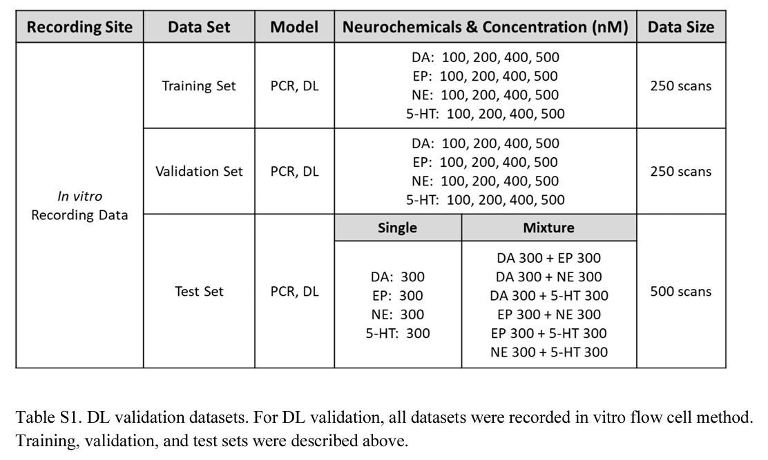
Data Processing
- After voltammograms were collected, signal processing including background subtraction and averaging was processed (MATLAB)
- For each concentration of each neurochemical, we collected 500 FSCV scans
- For the 100 nM, 200 nM, 400 nM, and 500 nM data sets, 250 of the voltammograms were used to build a training set of known analyte-concentration voltammograms
- The other half of these, and all of the 300 nM voltammograms, were used to build a validation and test data set
- To prevent overfitting and to ensure that we had sufficient data to train our model, we used data augmentation to artificially expand the data set by adding random noise to the signals
- We did not use input data flipping or scaling when augmenting the data due to the inherent importance of direction in the voltammogram
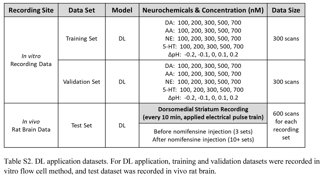
In Vivo Experiments for Deep Learning Model Applications
Analysis Methods
- PCR
- PCA → Create Regression Matrix → Predict
- Calculate residual threshold from the reconsturcted voltammograms and actual voltammogram and check the residuals were below the threshold (To validate the model)
- Deep Learning
- 1D convolutional neural network
- Small receptive fields of size 3 and a stride of one sample with a ReLU activation function.
- The output is padded with one sample to preserve the resolution after convolution
- The network training was carried out by optimizing the mean squared error loss fuction, and the batch size was set to 20
- Used dropout regularization
- Used Adam optimizer and the learning rate was 0.2
- 5-fold cross-validation was used to avoid overfitting and monitor the model’s performance on a randomly selected validation set.`

Leave a comment